Bayesian climbing grades

Introduction

In indoor sport climbing different routes to the top of the wall are put up by different route setters who are also given the task of awarding each climb a ‘grade’.

Giving a climb a grade allows climbers known what they are getting in to before they start a route; higher graded climbs can be scarier, could be trickier to climb safely, and novice climbers climbing on hard climbs could even pick up injuries.

But, naturally, grades are also a scoring system for climbers, who make it their goal to reach a certain grade!

What makes this more interesting is that a climb cannot be graded objectively, setters combine information about:

• The terrain the route is on: a climb on an overhanging wall will normally be graded harder
• What the holds and moves are like: smaller holds spaced further apart will typically be harder and sometimes climbs will contain very strenuous or physiologically improbable moves which will also add to the overall grade
• The amount of stamina required to get to the top of a climb: Some climbs are very sustained, while others contain long easy sections puncuated by difficult ‘crux’ moves

Because all setters are different their opinions on a particular route will vary and it is that variation which I am interested in modelling today.

This idea started out when I noticed that at my local climbing wall I could often climb a certain grade if it was set by two setters; ‘Median Mike’ and ‘Generous Greg’ (I’ve anonymised the setters!) but I would struggle/fail much more on climbs of the same grade if they were set by ‘Sandbag Steve’.

I wondered if I could collect a bunch of data about which climbs I could and could not do, and then construct a model to compute the ’true grade’ of a climb, taking into account who set the route (and possibly other information about the style of the climb, the terrain, etc.). Now, I never got around to collecting this dataset…so instead I am going to generate some fake data and try to construct a model which can recover the ‘biases’ of each setter.

An important caveat: Climbers and route setters can be touchy about the subject of grades! So just to say, grades don’t really matter, this is just a bit of fun :)

The Model

There are two interesting things about this modelling problem:

• The good news: We actually have more data than just whether the climb was climbed successfully or not. We can know how many attempts at a climb were made, e.g. “This 6c+ took four attempts before it was climbed successfully”
• The bad news: It’s a censored data problem. Practically, people aren’t going to try a climb more than some amount. For the data in this model I’ve assumed that after twenty attempts at a climb result in failure the hypothetical climber simply gives up.

With the number of attempts available we choose to model the data as follows

$$ \text{logit}^{-1}(p_{\text{success}, i}) \sim f(\text{grade}_i, x_i), $$

$$ \text{attempts} \sim \text{Geometric}(p_{\text{success}, i}), $$

$$ \text{observations}_i = \text{Censored}(\text{attempts}_i, \text{max}=20) , $$

where $f$ is some smooth function of the grade and possibly some other features, $x_i$ and $p_{\text{success}, i}$ is the probability of doing a climb on each attempt.

If we wanted to, we could also experiment with some other cumulant functions for translating $f$ to a probability, I’ll stick with the logistic function.

And actually, in the rest of what follows I’m going to assume the following simple structure

$$ f(\text{grade}_i, x_i) = \alpha + \beta \cdot \text{grade}_i. $$

If we had real data to work with then perhaps a more general function like a smoothing spline would be interesting but this form will sufficient for our purposes.

A geometric distribution is the natural choice since it expresses the distribution of the number of bernoulli trials (attempts at a climb) because we observe a success (climbing the route). But it is a big assumption that the probability of success doesn’t depend on the number of attempts already taken at a route. This is clearly unrealistic since people can train to complete routes by repeatedly trying and perfecting individual moves, it’s also significantly harder to complete a climb first attempt since you’re climbing into the unknown. A reasonably way around this would be to include a binary feature into $f$ indicating if it was a climbers first attempt, given enough data it might be possible to have the probability of success scale with number of attempts but then we’d need to write a more general likelihood function since this would violate the IID assumption for a geometric distribution.

You might have noticed that so far the identity of the setter hasn’t entered into the model. There are three paths we can take here:

1. Fully pooled: We can fit the model, as stated and simply ignore the ‘setter’ feature of each route. In this approach we cannot recover the setter bias values which went into generating the data, but it has the advantage of being simple!

2. Individual models: We can fit the model $S$ times, once per route setter. Here, we can try to recover the setter bias values, but each model fit will have approximately a $1/S$ the amount of data to train on (where $S$ is the number of route setters) and so we should expect them to be more uncertain

3. Hierarchical: We model the $\alpha$ and $\beta$ parameters as being different for each setter, but they are each influenced by a common ‘hyperprior’ which will tend to keep them ’not too far’ from each other. This ’not too far’ is parametrised by the hyperprior variance in our model, and then learnt as part of the model sampling process

I’m going to use the hierarchical model: it has the benefits of (1) since we can train on the entire dataset, and the benefits of (2) since we are explicitly treating setter’s data as being different, and allowing the model to decide how different.

Generating some fake data

import numpy as np
import pandas as pd
import matplotlib.pyplot as plt
import pymc as pm
from scipy.stats import geom
from scipy import optimize

I’ll model the grade as a continuous positive value, where integers between zero and twelve map to defined grades (’the french grade’ of a route):

grades_str = ["5+", "6a", "6a+", "6b", "6b+", "6c", "6c+", "7a", "7a+", "7b", "7b+", "7c", "7c+"]
grades_map = {i: g for i, g in enumerate(grades_str)}
grades = np.array(list(grades_map.keys()))

We’re going to simulate three different route setters for this problem, each is going to have a different bias.

Median Mike is the middle of the road, Generous Greg typically sets a bit easier than expected for the grade and Sandbag Steve’s routes are famously stiff.

setters = [
    "Sandbag Steve",
    "Median Mike",
    "Generous Greg",
]

setter_bias = {
    0: +0.9,
    1:  0.0,
    2: -0.3,
}

And to complete the data generation process we must, for each attempted route, randomly pick a setter and a grade. We then adjust the ’true grade’ to account for the setter’s bias and sample the number of attempts it will take to successfully climb the route, applying censoring if need be

def sigmoid(x):
    return 1 / (1 + np.exp(-x))

def p_success(grade):
    return sigmoid(grades[-1] // 2 - grade)

def generate_data(N: int) -> pd.DataFrame:
    setter_idx = np.random.choice(list(setter_bias.keys()), N)

    attempted_grade = np.maximum(
        np.random.normal(grades.mean(), 2, size=N).astype(int),
        0,
    )

    df = pd.DataFrame(
        data=np.stack([setter_idx, attempted_grade]).T,
        columns=["setter", "grade"]
    )

    df.loc[:, "adjusted_grade"] = df.grade + df.setter.apply(lambda s: setter_bias[s])

    df.loc[:, "attempts"] = [
        np.random.geometric(p=p_success(row["adjusted_grade"]))
        for _, row in df.iterrows()
    ]

    df.loc[:, "censored"] = df.attempts > 20
    df.loc[:, "censored_attempts"] = np.clip(df.attempts, 0, 20)

    return df

df = generate_data(500)

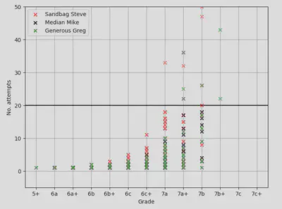
The resulting data is shown below with data point representing an individual climb, split by who set it. The transparent routes are the climbs on which we threw in towel, cursing the setter, blaming conditions and claiming to be having a “high gravity day” in the process:

Implementing the model

The model is straighforward to express in pymc:

coords = {"setters": [0, 1, 2]}

with pm.Model(coords=coords) as hierarchical_model:
    setter_idx = pm.Data("setter_idx", df.setter, dims="obs_id")
    grade_idx = pm.Data("grade_idx", df.grade, dims="obs_id")
    
    # Hyperpriors
    mu_a = pm.Normal("mu_a", mu=0.0, sigma=10.0)
    sigma_a = pm.Exponential("sigma_a", 5)
    mu_b = pm.Normal("mu_b", mu=0.0, sigma=10.0)
    sigma_b = pm.Exponential("sigma_b", 5)

    # Priors
    z_a = pm.Normal("z_a", mu=0, sigma=1, dims="setters")
    z_b = pm.Normal("z_b", mu=0, sigma=1, dims="setters")

    # Regression coefficients
    alpha = pm.Deterministic("alpha", mu_a + z_a * sigma_a, dims="setters")
    beta = pm.Deterministic("beta", mu_b + z_b * sigma_b, dims="setters")

    # The success probability for our geometric distribution
    p_success = pm.invlogit(alpha[setter_idx] + beta[setter_idx] * grade_idx)

    # The un-censored number of attempts to climb a route
    attempts = pm.Geometric.dist(p=p_success)

    # Applying the censoring and providing our observables
    pm.Censored(
        "censored_attempts",
        attempts,
        lower=0,
        upper=20,
        observed=df.censored_attempts,
    )

It is worth pointing out that I’m using a non-centered parametrisation for the alphas here to help the model sample efficiently. That is, I’m explicitly modelling the $\alpha$ and $\beta$ in terms of a $\mathcal{N}(0, 1)$ distribution, and then applying scaling and translation rather than directly modelling $\mathcal{N}(\mu, \sigma^2)$.

There’s a really interesting paper here ¹ which explains why such transforms help, and also talks a bit about how PPLs (STAN, pymc, Edward and co.) might be able to automatically re-parametrise models so that users can specify their models in whichever form they like without fear of trashing their effective sample sizes.

Sampling and analysis

We can sample from the model as follows:

with hierarchical_model:
    idata = pm.sample()

It takes less than a minute to run. The arviz package makes it very convenient to perform diagnostic checks on the inference data, after checking the traces (visually), the $\hat{R}$-values, ranks, ESS and MCMC chain marginal energies we can see that the NUTS sampler has done a good job.

The only concern is that the posterior-predictive mean misses the observed data by same margin…event though the posterior distribution itself describes the empirical value nicely:

with pooled_model:
    ppc = pm.sample_posterior_predictive(idata)

_, ax = plt.subplots(figsize=(12, 6))
az.plot_ppc(ppc, ax=ax)
ax.grid();

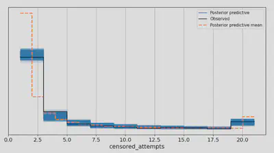
Odd! But I’m satisfied the inference data is OK so let’s proceed to some analysis.

Model analysis

We can start out just looking at the posterior mean values for our regression parameters:

alpha_hat = idata.posterior["alpha"].mean(("chain", "draw")).to_numpy()
beta_hat = idata.posterior["beta"].mean(("chain", "draw")).to_numpy()
alpha_hat, beta_hat
>>> (array([5.12205616, 5.80581224, 6.02555836]),
     array([-0.98364854, -0.96512455, -0.95451869]))

and we can use to look at the posterior predictive number of attempts, per setter, extrapolating to beyond the 20 attempts where the initial data was censored.

_, ax = plt.subplots(figsize=(8, 6))

def inv_logit(p):
    return np.exp(p) / (1 + np.exp(p))

xx = np.linspace(grades.min(), grades.max(), 100)

posterior_mean_p = inv_logit(alpha_hat[:, np.newaxis] + np.outer(beta_hat, xx))

for i in range(3):
    ax.scatter(
        df[(df.setter == i) & ~df.censored].grade, 
        df[(df.setter == i) & ~df.censored].attempts,
        marker='x',
        color=colors[i],
    )
    ax.scatter(
        df[(df.setter == i) & df.censored].grade, 
        df[(df.setter == i) & df.censored].attempts,
        marker='x',
        color=colors[i],
        alpha=0.2,
    )

for i in range(3):
    plt.plot(
        xx,
        geom(posterior_mean_p[i, :]).mean(),
        label=f"Posterior mean ({setters[i]})",
        color=colors[i],
    )
    
ax.axhline(20, color="black")
ax.legend()
ax.set_xticks(grades)
ax.set_xticklabels(grades_str)
ax.grid()
ax.set(ylim=(-5, 50), xlabel="Grade", ylabel="No. Attempts");

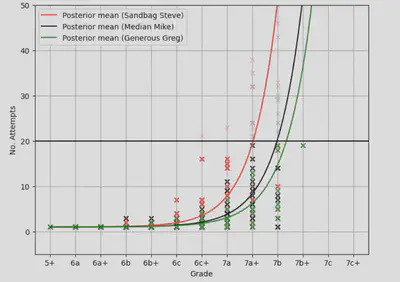
The posterior mean number of attempts seems to fit the data well and the sign of the setter biases matches that of the values used to generate the dataset.

But we should be using all of the information from the posterior!

This requires a little index trickery to compute conveniently, but it’s not so bad:

_, ax = plt.subplots(figsize=(12, 10), nrows=3)

posterior_mean_p = inv_logit(alpha_hat[:, np.newaxis] + np.outer(beta_hat, xx))

xx = np.linspace(grades.min(), grades.max(), 100)

a = idata.posterior["alpha"].mean(("chain")).to_numpy()
b = idata.posterior["beta"].mean(("chain")).to_numpy()

a = a[:, np.newaxis, :, np.newaxis]       # (100, 1, 3, 1)
b = b[np.newaxis, :, :, np.newaxis]       # (1, 100, 3, 1)
xx_broadcast = xx[np.newaxis, np.newaxis, np.newaxis, :]  # (1, 1,   1, 100)

p_samples = (inv_logit(a + b * xx_broadcast)).reshape(1000 * 1000, 3, 100)

posterior_mean_p = inv_logit(alpha_hat[:, np.newaxis] + np.outer(beta_hat, xx))

p_low, p_high = np.percentile(p_samples, [2.5, 97.5], axis=0)

for j in range(3):
    for i in range(3):
        ax[j].scatter(
            df[(df.setter == i) & ~df.censored].grade, 
            df[(df.setter == i) & ~df.censored].attempts,
            marker='x',
            color=colors[i],
        )
        ax[j].scatter(
            df[(df.setter == i) & df.censored].grade, 
            df[(df.setter == i) & df.censored].attempts,
            marker='x',
            color=colors[i],
            alpha=0.2,
        )

for j in range(3):
    for i in range(3):
        if i != j:
            continue
        ax[j].plot(
            xx,
            geom(posterior_mean_p[i, :]).mean(),
            label=f"Posterior mean + 95% CI ({setters[i]})",
            color=colors[i],
        )
        ax[j].fill_between(
            xx,
            geom(p_low[i, :]).mean(),
            geom(p_high[i, :]).mean(),
            color=colors[i],
            alpha=0.25
        )

[a.axhline(20, color="black") for a in ax.ravel()]
[a.legend() for a in ax.ravel()]
[a.set_xticks(grades) for a in ax.ravel()]
[a.set_xticklabels(grades_str) for a in ax.ravel()]
[a.grid() for a in ax.ravel()]
[a.set(ylim=(-5, 50), ylabel="No. Attempts") for a in ax.ravel()]
ax[-1].set(xlabel="Grade");

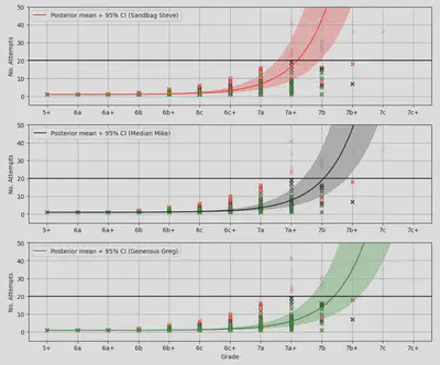
Arguably there is some model over-confidence at the low end of the grade range, but generally the posterior uncertainty captures the data well.

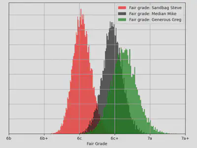
It is interesting to ask what the “fair grade” of a climber is. This has been defined, in other quantitative studies on climbing, as the grade at which a given climber has a 50% chance of climbing a route on the first attempt.

Focusing on the posterior mean first:

def fair_grade(alpha, beta):
    def _fair_grade(xx, alpha, beta):
        return inv_logit(alpha + beta * xx) - 0.5

    sol = optimize.root_scalar(
        _fair_grade,
        bracket=[grades.min(), grades.max()],
        method='brentq',
        args=(alpha, beta)
    )
    return sol.root

for i in range(3):
    fg = fair_grade(alpha_hat[i], beta_hat[i])
    print(f"{setters[i]} -> {fg:.4f} -> {grades_map[round(fg)]}")

>>> Sandbag Steve -> 5.0752 -> 6c
>>> Median Mike   -> 5.9348 -> 6c+
>>> Generous Greg -> 6.2476 -> 6c+

So Steve’s harder setting is worth, approximately, half a grade compared with Mike and Greg. The posterior plots above suggest that the model can see that Greg sets easier routes than Mike, but when we round back the discretised French grade system, both come out as “6c+”. If we look at the full posterior for the fair grade we can see the difference (note that I’m down-sampling the MCMC chains here just to get this to run in a reasonable amount of time):

from collections import defaultdict
from itertools import product

a = idata.posterior["alpha"].mean(("chain")).to_numpy()
b = idata.posterior["beta"].mean(("chain")).to_numpy()

a_samples = a[1::10,:]
b_samples = b[1::10,:]

values = defaultdict(lambda: np.zeros(a_samples.shape[0] * b_samples.shape[0]))

for i in range(3):
    for j, (α, Β) in enumerate(product(a_samples[:,i], b_samples[:,i])):
        fg = fair_grade(α, Β)
        values[i][j] = fg

_, ax = plt.subplots(figsize=(8, 6))
for i in range(3):
    ax.hist(
        values[i],
        bins=100,
        label=f"Fair grade: {setters[i]}",
        alpha=0.7,
        color=colors[i],
        density=True,
    )

ax.set_xticklabels(grades_str)
ax.grid()
ax.set_xticks(grades[3:9], [grades_map[g] for g in grades[3:9]])
ax.set(xlabel="Fair Grade")
ax.grid(True)
ax.legend()
ax.yaxis.set_ticks_position('none')
ax.yaxis.set_ticklabels([]);

And finally, we can re-frame the above data to study the posterior for ‘setter bias’, using Median Mike as the reference setter:

_, ax = plt.subplots(figsize=(8, 6))

ax.hist(values[0] - values[1], color=colors[0], alpha=0.7, label="Steve sampled bias", bins=100)
ax.hist(values[2] - values[1], color=colors[2], alpha=0.7, label="Greg sampled bias", bins=100)
ax.set(xlabel="Grade Bias")
ax.axvline(-0.9, color=colors[0], label="Steve's true bias")
ax.axvline(+0.3, color=colors[2], label="Greg's true bias")
ax.grid(True)
ax.legend()
ax.yaxis.set_ticks_position('none')
ax.yaxis.set_ticklabels([]);

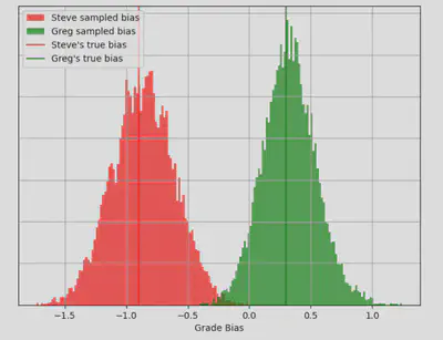
Nice! The model has been able to recover the biases I used to generate the dataset nicely.

The obvious next question is how many times would I have to climb ‘Silence 9C’ ², the hardest route in the world at the time of writing…Well of course, it depends if you believe Greg, Mike or Steve!

geom(inv_logit(alpha_hat + 19 * beta_hat)).mean()
>>> array([1038116.2991997 ,  300767.01037835,  177902.1097564 ])

Only 178 thousand attempts!

References