Cublic Spline Expansions with Logistic Regression

This is an example from chapter 5 (‘Basis Expansions and Regularisation’) of the excellent Elements of Statistical Learning book ¹. It’s section 5.2.3 - ‘Phoneme Recognition’.

The dataset ² contains 1717 examples of periodogram data for different test subjects saying the letter combinations such as “ao” and “aa”. Periodograms are not something I am familiar with, but a little research suggests they are quite similar to the discrete Fourier transform. The periodograms we have have been log-transformed, and each contains 256 frequencies.

Our task then, is to predict which letter combination was spoken, given the 256 datapoints we have for the intensity of each frequency. I.e. this is a binary classification problem.

Here, I’ll first train a simple logistic regression model on the full dataset, treating each frequency as an independent feature and then, following along with the textbook, try a more interesting model class.

Since the phonemes are naturally produced sounds it is reasonable to expect that the frequency profiles be smooth functions and, therefore, we would expect that the regression coefficients for some frequency, $f$, be quite close to that of $f+1$ and $f-1$. But to the simple logistic regression model they are just labels and the features $(f, f+1, f-1)$ bear no relation to one another so far as it is concerned. Therefore we realise that the logistic regression model using the raw features as inputs isn’t physically well motivated and instead we choose to first perform a basis expansion using cubic polynomials, and then perform logistic regression where the coefficients are those of the polynomials.

First things first - let’s start out with the imports we need…

import numpy as np
import pandas as pd
from scipy.stats import norm
from scipy.special import expit
import matplotlib.pyplot as plt

from patsy import cr as natural_cubic_basis

from sklearn.pipeline import Pipeline, FunctionTransformer
from sklearn.linear_model import LogisticRegression
from sklearn.dummy import DummyClassifier
from sklearn.metrics import accuracy_score
from sklearn.model_selection import train_test_split, cross_val_score

import pymc as pm
import arviz as az
from pymc.math import sigmoid

…and perform a little data wrangling:

def binary_encode_categorical(target_column: pd.Series) -> pd.Series:
    unique_values = target_column.unique()
    if unique_values.shape[0] > 2:
        raise RuntimeError("Your categorical feature doesn't look binary")
    return pd.get_dummies(target_column)[unique_values[0]]

N = 256
XX = range(N)

target_name = "phoneme"

# Rename some columns with more descriptive names
# (and remove dots which don't play nicely with the pandas API)
target_renaming_dict = {"g": target_name}
feature_renaming_dict = {f"x.{i}": f"x_{i}" for i in range(1, N + 1)}

df = (
    pd.read_csv("phoneme_recognition.csv")
    # We don't need the index or the ID of the phoneme speaker
    .drop(["row.names", "speaker"], axis=1)
    .rename(columns={**target_renaming_dict, **feature_renaming_dict})
    # Two outcome classification problem as posed in the ESL book
    .query("phoneme in ('ao', 'aa')")
    .reset_index(drop=True)
)

# Encode the target variable as an integer
df.phoneme = binary_encode_categorical(df.phoneme)

with pd.option_context("display.max_columns", 7):
    display(df.head())

We can have a look at the shape of the data we are working with, and observe that it matches the plots from the book well:

Lastly, before we start building an actual model let’s make a quick dummy classification to get a baseline for what the more complex models should be aiming to beat:

dummy = DummyClassifier().fit(X_train, y_train)
dummy_accuracy = accuracy_score(dummy.predict(X_test), y_test)
print(dummy_accuracy)
>>> 0.5648535564853556

56%, barely better than a random guess, so this should be beatable!

Logistic regression on the raw data

We’ll be interested in the out-of-sample error of our models so we choose to split our data into separate train and test sets:

features_names = list(feature_renaming_dict.values())

X_train, X_test, y_train, y_test = train_test_split(
    df[features_names].values,
    df[target_name].values,
    train_size=1000
)

The logistic regression model working with the raw frequencies is fitted as follows:

logit = LogisticRegression(max_iter=1e6)

shuffle_idx = np.random.choice(XX, len(XX), replace=False)
logistic_model = logit.fit(X_train[:, shuffle_idx], y_train)

raw_train_accuracy = accuracy_score(logistic_model.predict(X_train[:, shuffle_idx]), y_train)
raw_test_accuracy = accuracy_score(logistic_model.predict(X_test[:, shuffle_idx]), y_test)

print(raw_train_accuracy, raw_test_accuracy)
>>> 0.929 0.7391910739191074

Already a pretty good accuracy score and as we would hope, this outperforms the dummy classifier which completely ignored all of the information in the feature set. Also not that these accuracies are pretty similar to those quoted in ¹.

The shuffle_idx trick is simply rearranging the features randomly (consistently across both the training and test set). There’s no actual point to this beyond driving home the point that the logistic regression really doesn’t care that neighbouring frequencies are related - any choice or reordering will result in identical models.

Cubic spline smoothed logistic regression

Now let’s try something fancier. Since, as discussed above, the log-periodograms are smooth functions we’ll try to express them as a linear combination of cubic basis functions. We can see the sorts of functions this results in by building a basis using the patsy python package and randomly generating some coefficients for them:

_, ax = plt.subplots(figsize=(10, 10), nrows=3)

coeffs = np.abs(np.random.normal(size=basis.shape[1]))
basis = natural_cubic_basis(XX, df=6)

ax[0].plot(XX, basis)
ax[1].plot(XX, basis * coeffs)
ax[2].plot(XX, basis * coeffs, alpha=0.4)
ax[2].plot(XX, basis @ coeffs, lw=3, color="black")

ax[2].set(xlabel="x")
ax[1].set(ylabel="y");

When generating the basis we requested six degrees of freedom (The unfortunately named df variable) and this corresponds to the 6 cubic basis functions we have in the first plot. These are our building blocks which, when combined with some weights, can be scaled (second plot) and then summed (third plot). If we choose a higher number of degrees of freedom we could build increasingly ‘wiggly’ functions.

Our model is now in two steps - we first express the features in terms of the basis function (refered to as the $H$ matrix in ¹) and then we perform the logistic regression using the basis weights as features:

def build_cubic_spline_regression(basis: np.array, **lr_kwargs):
    return Pipeline(
        [
            ("spline_tranform", FunctionTransformer(lambda X: X @ basis)),
            ("regression", LogisticRegression(max_iter=1e6, **lr_kwargs)),
        ]
    )

But now we have a problem we didn’t have when we ran the regression on the raw frequencies - how many terms, df, is the correct number to include in our basis expansion? We can run the model with a few different sizes of basis (4, 12 and 36) and inspect the solutions visually:

_, axs = plt.subplots(figsize=(12, 16), nrows=3)

for i, df in zip(range(3), [4, 12, 36]):
    basis = natural_cubic_basis(XX, df=df)
    model = build_cubic_spline_regression(basis).fit(X_train, y_train)

    ax, ax2 = axs[i], axs[i].twinx()
    h1 = ax.plot(
        XX,
        logistic_model.coef_.ravel(),
        color="b",
        label="Raw logistic regression coefficients",
    )
    h2 = ax2.plot(
        XX,
        basis @ model.named_steps['regression'].coef_.ravel(),
        color="r",
        label=f"Cubic spline logistic regression spline (dof = {df})",
    )
    ax.axhline(0)
    ax.set(xlabel='Frequency', ylabel='Coeff.')
    ax.legend(handles=h1 + h2)

Included in blue are the coefficients of raw logistic regression model for comparison and we can now see visually that the original model leads to a very ‘spiky’ results. In some cases the model has learned that neighbouring frequencies actually have opposite effects on the log-odds in some cases (because the sign of the coefficients has flipped).

When the model is only allowed 4 degrees of freedom it appears to be underfitting the data. When df = 12 starts to look a bit more reasonable and by the time we’re at the most complex model we might start to suspect we’re overfitting - and therefore that the resulting model might not generalise well when predicting on new data.

Cross validation to optimise the spline basis

Of course, we can do better than just looking at fitted coefficients to choose the size of the basis function. We can use cross-validation to try and estimate the out-of-sample model error for a range of different basis functions and select the model which performs the best:

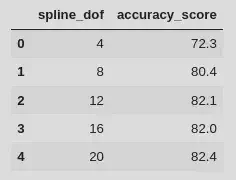
dofs = np.linspace(4, 20, 5, dtype=int)
scores = np.zeros(dofs.size)

for i, dof in enumerate(dofs):
    basis = natural_cubic_basis(XX, df=dof)
    model = build_cubic_spline_regression(basis)
    cv_scores = cross_val_score(model, X_train, y_train, cv=10, scoring="accuracy")
    scores[i] = cv_scores.mean()

df_cv = pd.DataFrame(
    data=np.array([dofs, 100 * scores]).T,
    columns=["spline_dof", "accuracy_score"]
)

df_cv.spline_dof = df_cv.spline_dof.astype(int)

display(df_cv)

_, ax = plt.subplots(figsize=(10, 6))

ax.axhline(
    df_cv.iloc[df_cv.accuracy_score.idxmax()].accuracy_score,
    color="b",
    ls="--",
    label="Best Spline Logistic Regression accuracy score"
)
ax.axvline(df_cv.iloc[df_cv.accuracy_score.idxmax()].spline_dof, color="b", ls="--")
ax.scatter(df_cv.spline_dof, df_cv.accuracy_score, color="b", marker="x")
ax.axhline(
    100 * raw_test_accuracy,
    color="red",
    ls="--",
    label="Best Raw Logistic Regression accuracy score"
)
ax.axhline(
    100 * dummy_accuracy,
    color="black",
    ls="--",
    label="Dummy classified accuracy score"
)
ax.set(xlabel="Spline dof", ylabel="Cross validation accuracy (%)")
ax.legend();

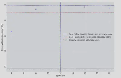
The most complex has the highest cross-validation accuracy score, but df=12 performs almost as well and has around half the number of parameters - given this, I would probably tend to choose the df=12 model, it’ll run faster etc. With the optimal basis size choosen we can compare its performance to the raw regression model:

basis = natural_cubic_basis(XX, df=12)
model = build_cubic_spline_regression(basis).fit(X_train, y_train)
spline_train_accuracy = accuracy_score(y_train, model.predict(X_train))
spline_test_accuracy = accuracy_score(y_test, model.predict(X_test))

pd.DataFrame(
    data=[
        [raw_train_accuracy, raw_test_accuracy],
        [spline_train_accuracy, spline_test_accuracy],
    ],
    index=["Raw Logistic Regression", "Cublic Spline Logistic Regression"],
    columns=["Training Set Accuracy", "Test Set Accuracy"],
).T

Nice! The raw logistic regression model outperforms the spline version by 10% on the training data but it generalises quite poorly and we find that the best option is the cubic spline logistic regression.

Bayesian Cubic Spline Logistic Regression

Taking this a step further we can perform a bayesian logistic regression with the same cubic basis function expansion as above. The advantage then is that we can produce credible intervals for the spline coefficients and the make stataments about our uncertainty on the logistic probabilities too.

These models are straightforward to express using the pymc probibilistic modelling package ³.

The raw logistic regression model first:

with pm.Model() as raw_logistic_model:
    weights = pm.Normal("weights", 0, 1e1, shape=X_train.shape[1])
    pm.Bernoulli(
        "logit",
        p=sigmoid(pm.math.dot(X_train, weights)),
        observed=y_train,
    )

I have choosen a fairly tight prior for the logistic regression weights here, but we know these values are quite close to zero from the non-bayesian analogue above so I believe this is OK.

This model takes a very long time to sample MCMC chains from because it has 256 weights to fit (though, in fairness to pymc I am running this on a laptop…) but we can quickly fit the MAP estimate and look at the accuracy of that model:

with raw_logistic_model:
    map_estimate = pm.find_MAP()

map_predict = lambda XX: (expit(XX.dot(map_estimate["weights"])) > 0.5).astype(int)

print(
    accuracy_score(map_predict(X_train), y_train),
    accuracy_score(map_predict(X_test), y_test),
)
>>> 0.935 0.7308228730822873

Encouragingly, these are very close to the original model results: If the priors I’ve selected are not too overbearing then the MAP sould be close to the maximum likelihood estimates, which is what sklearn’s LogisticRegression was producing above.

Moving on to the cubic spline version:

with pm.Model() as spline_logistic_model:
	transformed_X = X_train @ natural_cubic_basis(XX, df=12)
    weights = pm.Normal("weights", 0, 1e1, shape=transformed_X.shape[1])
    pm.Bernoulli(
        "logit",
        p=sigmoid(pm.math.dot(X_train, weights)),
        observed=y_train,
    )
    trace = pm.sample(cores=4, draws=1000, return_inferencedata=True)

This time we have fewer parameters and the model fits very quickly. The arviz ⁴ package provides several diagnostics for checking that the model has fitted correctly - the Gelman-Rubin diagnostic ($\hat{R}$) and the Bayesian Fraction of Missing Information (BFMI) both look good in this case.

We can view the posterior distributions of each coefficient in our cubic basis if we like, but it’s more interesting to use those distributions to generate a range of basis expansions and look at those instead.

First we need to do a little manipulation to get the MCMC traces into numpy (they are returned as aesara objects by default) and then flatten them to combine the chains run on separate cores into one:

np_trace = trace["posterior"]["weights"].to_numpy()
np_trace = np_trace.reshape(-1, 12)

_, ax = plt.subplots(figsize=(12, 12), nrows=2)

basis = natural_cubic_basis(XX, df=12)
cubics = basis @ np_trace.T
mean_cubic = basis @ np_trace.mean(axis=0)

ax[0].plot(XX, mean_cubic, color="b", label="Mean regression")
ax[0].plot(XX, cubics[:,::20], color="b", alpha=0.05)
ax[0].set(xlabel="Frequency", ylabel="Coeff")

lower5, upper5 = np.percentile(cubics, [5, 95], axis=1)
ax[1].fill_between(XX, lower5, upper5, color="b", alpha=0.1, label="95% credible interval")
ax[1].plot(XX, mean_cubic, color="b", label="Mean")
ax[1].set(xlabel="Frequency", ylabel="Coeff")

[a.legend() for a in ax];

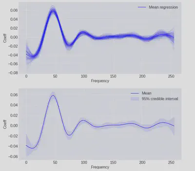
Here we can see the individual spline expansions from each of the steps in the MCMC trace in the first plot and the 95% credible intervals of those traces in the second plot.

We can also use these weights to produce distributions for the logistic probabilities for specific examples in the dataset:

_, ax = plt.subplots(figsize=(12, 4), ncols=2)
ax[0].hist(expit(np_trace @ transformed_X[10, :]), bins=50, density=True, color="b", alpha=0.9, label="Ground truth = 0")
ax[1].hist(expit(np_trace @ transformed_X[21, :]), bins=50, density=True, color="b", alpha=0.9, label="Ground truth = 1")
[a.set(xlim=(0, 1)) for a in ax];

Having a measure of uncertainty here could be very useful, and this is one of the main advantages to taking a Bayesian modelling approach. For example, if the cost of misclassifying y=0 as 1 was very high then we might choose to ignore the model if the posterior predictive distribution had high variance.

Bayesian Model Selection

There is one last fun thing we can do here. In the above pymc model definition I quietly continued using a basis with twelve degrees of freedom because of the cross-validation performed. But with a Bayesian model we now have another option.

With our non-Bayesian logistic regression we used sklearn’s cross_val_score function which follows the usual k-fold cross-validation strategy of splitting the data into chunks, then training and testing repeatedly, changing which chunk was the test set each time. It’s quick to run in that case because the logistic regression will be using something like iteratively re-weighted least squares to train and that wil converge quickly.

However, with our Bayesian model retraining is relatively expensive - each model takes a few minutes on my laptop. Based on that figure, if we wanted to do a full leave-one-out (LOO) cross-validation it would take $\mathcal{O}(\text{one week})$ to run! Luckily the Bayesian model allows us to use a modern idea with the catchy name LOO-PSIS cross-validation (Leave-One-Out Pareto Smoothed Importance Sampling cross-validation) - it’s complicated and I don’t trust my understanding enough to commit it to writing here – please refer to this paper ⁵ for details. PSIS-LOO allows us to get an approximation of the generalisation error of each model without having to retrain the model at all, which is pretty incredible!

In code (plot_compare referenced below was lifted verbatim from an excellent Austin Rochford piece ⁶):

traces = {}

for bs in (4, 8, 12, 16, 20):
    with pm.Model() as full_logistic_model:
    transformed_X = X_train @ natural_cubic_basis(XX, df=bs)
        weights = pm.Normal("weights", 0, 1e1, shape=transformed_X.shape[1])
        pm.Bernoulli(
            "logit",
            p=sigmoid(pm.math.dot(X_train, weights)),
            observed=y_train,
        )
        traces[bs] = pm.sample(cores=4, draws=1000, random_seed=[1, 2, 3, 4], return_inferencedata=True)

loo_df = az.compare(traces, ic="loo", seed=1234)
display(loo_df)
plot_compare(loo_df, "LOO");

Higher values for log-score are better here. So this confirms the findings of the cross-validation study from above: 12 degrees of freedom gets you the best bang for your buck!

References