The EM Algorithm Part 2: Censored Linear Regression

Introduction

This is a follow up to part 1 ¹ in which we went through the theory required for the Expectation-Maximisation alogorithm and applied it to fit a gaussian mixture model.

In part 2 we’ll use the EM alogorithm on a different class of problem. Here, we’ll look at the problem of linear regression with ‘censored’ data. Data censoring is a type of missing data problem where the dependent variable of a data point is unobserved. A macabre, but common, example of data censoring occurs in studies of medical trials.

Say we were studying the effect of an experimental drug on an incurable deadly disease. We would probably assign patients a unique identfier, record whether they were taking a placebo or the real experimental drug and then wait to observe the time taken for the disease to kill them. The problem is that our trial can’t go on indefinitely while we wait for everyone in the trial to die - and so it’s likely that a proportion of patients will survive longer than our trial lasts and therefore we will never get a full observation of that data point. We could choose to just not include such patients in our study, but then we are throwing away the information that they survived.

So then, the question is how can we best include censored data.

I recommend the following text books on this subject ^{2 3 4 5}.

Data generation and vanilla OLS

Let’s come up with a toy dataset to play with:

# Generate linearly related data and add a noise term
N = 100
b0, b1 = 3.0, 0.2
xx = np.linspace(0, 10, N)
xx += np.random.normal(0, 0.5, N)
yy_uncensored = b0 + b1 * xx + np.random.normal(0, 0.2, N)

# Define an arbitrary cut-off above which points will be truncated
truncation_line = 0.15 + b0 + (b1 - 0.05) * xx

# Censor the data:
censored = yy_uncensored > truncation_line
yy = np.where(censored, truncation_line, yy_uncensored)

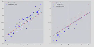
As you can see a subset of the data has been censored above some arbitrary slice through the x-y plane. A significant amount has been removed, nearly 70%. There are two naive things we can try straight away:

• Bad idea 1: We can just ignore the data, remove the censored points and perform an ordinary least squares (OLS) regression,
• Bad idea 2: We could take the censored $y$ values as the true $y$ values.

Both of these approaches are shown below (“Bad idea 1” and “Bad idea 1” resp.), compared with the true regression line:

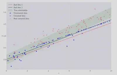
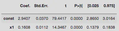
Visually these are both poor fits. The OLS regression coefficients, obtained using statsmodels, are shown below.

Bad idea 1:

Bad idea 2:

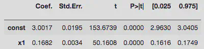
The first version’s constant term doesn’t contain the true value within $1\sigma$, whereas the second attempt just about does. Both of them badly underestimate the linear coefficient. So let’s try something better.

EM with censored data

The model we’ll build is only allowed to know the $x$ value for these censored points and the lower bound for their $y$ value. The true, unobserved, $y_i$ values will be represented in the model by the latent variables $z_i$. Based on the probabilistic interpretation of OLS we can write down our model as:

\begin{align*} y_i &\sim \mathcal{N}(\beta_0 + \beta_1 x_i, \sigma^2), \newline z_i &\sim \mathcal{N}(\beta_0 + \beta_1 x_i, \sigma^2). \end{align*}

With this we can proceed with the E-step of the EM algorithm and write down the $\mathcal Q$ function for this problem. Assuming there are $N_c$ censored data points:

\begin{align*} \mathcal{Q}(\theta|\theta_n) = \mathbb{E}_{z_i|x_i, \theta_n}\left[\log \prod_ip(x_i, z_i| \theta_n)\right], \newline \end{align*}

\begin{align*} = \mathbb{E}_{z_i|x_i, \theta_n}\Bigg[\log \Bigg(\prod_{i=0}^{N_c}\frac{1}{\sqrt{2\pi\sigma^2}} \exp(-\frac{1}{2\sigma^2}(x - \beta_0 - \beta_1x_i)^2) \ldots \newline \prod_{i=N_c}^{N}\frac{1}{\sqrt{2\pi\sigma^2}}\exp(-\frac{1}{2\sigma^2}(x - \beta_0 - \beta_1x_i)^2)\Bigg)\Bigg], \newline \end{align*}

\begin{align*} = - &\frac{N}{2}\log2\pi\sigma^2 - \frac{1}{2\sigma^2}\sum_{i=0}^{N_c}(y_i-\beta_0-\beta_1x_i)^2 - \ldots\newline & \mathbb{E}_{z_i|x_i, \theta_n}\Big[\frac{1}{2\sigma^2}\sum_{i=N_c}^N(z_i-\beta_0-\beta_1x_i)^2\Big], \newline \end{align*}

\begin{align*} = - &\frac{N}{2}\log2\pi\sigma^2 - \frac{1}{2\sigma^2}\sum_{i=0}^{N_c}(y_i-\beta_0-\beta_1x_i)^2 - \ldots\newline & \frac{1}{2\sigma^2}\sum_{i=N_c}^N(\mathbb{E}_{z_i|x_i, \theta_n}[z_i^2] - 2z_i\beta_0 - 2\beta_1x_i\mathbb{E}_{z_i|x_i, \theta_n}[z_i]+\beta_0^2+\beta_1^2x_i^2) \end{align*}

Ok, now for the M-step. We need to find the parameters which maximise $\mathcal{Q}$. For $\sigma^2$

\begin{align*} \frac{d\mathcal{Q}}{d\sigma^2} = - \frac{N}{2\sigma^2} + \frac{1}{2\sigma^4}\sum_{i=0}^{N_c}(y_i-\beta_0-\beta_1x_i)^2 + \frac{1}{2\sigma^4}\sum_{i=0}^{N_c}(z_i-\beta_0-\beta_1x_i)^2, \end{align*}

\begin{align*} \Rightarrow \hat\sigma^2 = \frac{1}{N}\Big(\sum_{i=0}^{N_c}(y_i-\beta_0-\beta_1x_i)^2 + \sum_{i=0}^{N_c}(y_i-\beta_0-\beta_1x_i)^2\Big). \end{align*}

For $\beta_0$

\begin{align*} \frac{d\mathcal{Q}}{d\beta_0} = \frac{1}{\sigma^2}\sum_{i=0}^{N_c}(y_i-\beta_0-\beta_1x_i) + \frac{1}{\sigma^2}\sum_{i=N_c}^N(z_i-\beta_0-\beta_1x_i) = 0, \newline \end{align*}

\begin{align*} \Rightarrow \hat\beta_0 = \frac{1}{2N}\left(\sum_{i}^{N_c} y_i + \sum_{i=N_c}^{N} z_i\right) - \beta_1\bar X. \newline \end{align*}

For $\beta_1$

\begin{align*} \frac{d\mathcal{Q}}{d\beta_1} = \frac{1}{\sigma^2}\sum_{i=0}^{N_c}x_i(y_i-\beta_0-\beta_1x_i) + \frac{1}{\sigma^2}\sum_{i=N_c}^Nx_i(z_i-\beta_0-\beta_1x_i) = 0, \newline \end{align*}

\begin{align*} 0 = \sum_{i=0}^{N_c}x_iy_i-2N\beta_0\overline{x}-2\beta_1\sum_{i=0}^{N_c}x_i^2, \end{align*}

and substituting in for $\beta_0$

$$ \hat\beta_1 = \frac{1}{\sum_{i=0}^N x_i - N\bar{x}^2}\left(\sum_{i=0}^{N_c} x_iy_i+ \sum_{i=N_c}^N x_iz_i - \bar{x}\left(\sum_{i=0}^{N_c} y_i + \sum_{i=N_c}^N z_i\right)\right). $$

So all that is left is to compute the expected values for the latent variables, $z$. we note that they must follow a truncated normal distribution, bounded below by the censored time of each observation

$$ p(z_i | x_i, \beta_0, \beta_1, \sigma^2) = \mathcal{TN}(\beta_0 + \beta_1x_i, \sigma^2, z_i \geq c_i) $$

where $c_i$ is the censored time for each point. For the E step of the EM algorithm we need to compute the folling expectations involving the latent variables:

\begin{align*} \mathbb{E}(z_i | x_i, \beta_0, \beta_1, \sigma^2) = \beta_0 + \beta_1x_i + \frac{\varphi(z_i | x_i, \beta_0, \beta_1, \sigma^2)}{1 - \Phi(z_i | x_i, \beta_0, \beta_1, \sigma^2)}, \newline \end{align*} \begin{align*} \mathbb{E}(z_i^2 | x_i, \beta_0, \beta_1, \sigma^2) = &(\beta_0 + \beta_1x_i)^2 + \sigma^2 + \ldots\newline &\sigma^2(\beta_0 + \beta_1x_i)\frac{\varphi(z_i | x_i, \beta_0, \beta_1, \sigma^2)}{1 - \Phi(z_i | x_i, \beta_0, \beta_1, \sigma^2)} \end{align*}

where $\varphi$ and $\Phi$ are the pdf and cdf of a standard normal distribution, respextively.

Ok, we have all of the ingredients we need to compute the regression coefficients for our toy data:

def mu(b0, b1, x_i):
    return b0 + b1 * x_i


def expectation_z_i(xx, yy, b0, b1, sigma2, censored):
    mu_ = mu(b0, b1, xx[censored])
    norms = stats.norm(mu_, np.sqrt(sigma2))
    pdfs = norms.pdf(yy[censored])
    cdfs = norms.cdf(yy[censored])
    return mu_ + sigma2 * pdfs / (1.0 - cdfs)


def expectation_z2_i(xx, yy, b0, b1, sigma2, censored):
    mu_ = mu(b0, b1, xx[censored])
    norms = stats.norm(mu_, np.sqrt(sigma2))
    pdfs = norms.pdf(yy[censored])
    cdfs = norms.cdf(yy[censored])
    return mu_ ** 2 + sigma2 + sigma2 * (yy[censored] + mu_) * pdfs / (1.0 - cdfs)


def mle_update_b0(n, b0, b1, xx, yy, zz, zz2, censored):
    return ((yy[~censored].sum() + zz.sum()) / n) - b1 * xx.mean()


def mle_update_b1(n, b0, b1, xx, yy, zz, zz2, censored):
    a = (xx[~censored] * yy[~censored]).sum() + (xx[censored] * zz).sum()
    b = xx.mean() * (yy[~censored].sum() + zz.sum())
    c = (xx ** 2).sum() - n * xx.mean() ** 2
    return (a - b) / c


def mle_update_sigma2(n, b0, b1, xx, yy, zz, zz2, censored):
    mu_censor = mu(b0, b1, xx[ censored])
    mu_event = mu(b0, b1, xx[~censored])
    return (
        ((yy[~censored] - mu_event) ** 2).sum() + (zz2 - 2.0 * mu_censor * zz + mu_censor ** 2).sum()
    ) / n


N = xx.shape[0]
b0, b1, sigma2 = 1, 1, 1

for itr in range(100):
    # E-step
    zz  = expectation_z_i (xx, yy, b0, b1, sigma2, censored)
    zz2 = expectation_z2_i(xx, yy, b0, b1, sigma2, censored)

    # M-step
    b1 = mle_update_b1(N, b0, b1, xx, yy, zz, zz2, censored)
    b0 = mle_update_b0(N, b0, b1, xx, yy, zz, zz2, censored)
    sigma2 = mle_update_sigma2(N, b0, b1, xx, yy, zz, zz2, censored)

b0, b1, np.sqrt(sigma2)

>> (2.966255608980418, 0.2153640423869373, 0.20832058429495817)

Pretty good! As a reminder the true values were $\beta_0=3.0$ and $\beta_1=0.2$. Let’s visually compare the solution against the two bad ideas tried earlier.

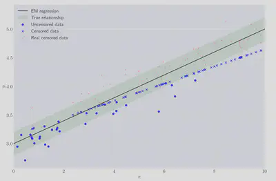
At this point it’s worth remembering that the EM regression has only seen the blue data in the right hand plot, and yet it’s a little hard to see the EM regression line because it’s almost on top of the true regression line, pretty great!

Bonus section: Fitting censored regression with pymc

This section has nothing to do with the EM algorithm, but it’s another interesting way to approach the same problem so I thought it was worth a mention. Earlier we wrote down the probabilistic form for an OLS regression:

$$ y_i \sim \mathcal{N}(\beta_0 + \beta_1 x_i, \sigma^2). $$

We can use an approach called Markov Chain Monte Carlo (MCMC) to find the posterior distributions for $\beta_0$ and $\beta_0$. A full description of how MCMC works is beyond the scope of this brief section but there are plenty of great references out there (see the references included below). For now it’s enough to know that MCMC is a method for approximating posterior distributions in Bayesian statistical models by cleverly traversing random paths through the parameter space of the model. pymc ⁶ is a python package built on top of theano which makes building and sampling from models very convenient.

First let’s try to fit a Bayesian OLS regression where we ignore the censored data:

import pymc as pm
from aesara import tensor as T

def fully_observed_normal_likelihood(
    mu: T.TensorVariable,
    sigma: T.TensorVariable,
    yy: np.array,
) -> T.TensorVariable:
    return T.sum(
        pm.logp(pm.Normal.dist(mu, sigma), yy)
    )

with pm.Model() as model:
    beta = pm.Normal('beta', 0.0, 100.0, shape=2)
    sigma = pm.HalfCauchy('sigma', 100.0)
    mu = beta[0] + xx * beta[1]
    likelihood = fully_observed_normal_likelihood(mu, sigma, yy)
    pm.Potential("likelihood", likelihood)
    idata = pm.sample(4000)

(those familiar with pymc will note that I’ve expressed the model in a slightly odd way – I’ve done this to make the censored version, below, clearer)

And that is all we need! The inference data variable, idata, contains details of the MCMC paths which were taken for each variable. There are lots of sanity checks which can (and should!) be performed on these traces to ensure that the model has converged well but here I’ll just show the posterior distributions:

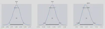
The highest posterior density (HPD - also known as the ‘credible interval’) regions are indicated for each variables - these are similar to the frequentist ideal of confidence internals for fitted model parameters. As before when we ran a non-Bayesian OLS, the parameters are not in good agreement with the true values. $\beta_0$ is just about contained in the credible interval, but $\beta_1$ and $\sigma$ both underestimate their actual values.

Luckily it’s possible to do better. We need to construct the following log-probability expression for the censored data ⁷

$$ \log p(y > c_i) = \log\int_{c_i}^\infty\mathcal{N}(y|\mu, \sigma)dy = \log\left(1 - \Phi\left(\frac{c_i - \mu}{\sigma}\right)\right), $$

and for the fully observed data we simply sample from a standard normal, as seen in fully_observed_normal_likelihood above. We can achieve this using aesara’s switch function, which behavious like a python if/else block, or numpys where function:

from pymc.distributions.dist_math import normal_lccdf

def right_censored_likelihood(
    is_censored: T.TensorConstant,
    mu: T.TensorVariable,
    sigma: T.TensorVariable,
    yy: np.array,
) -> T.TensorVariable:
    return T.sum(
        T.switch(
            T.eq(is_censored, 1),
            normal_lccdf(mu, sigma, yy),
            pm.logp(pm.Normal.dist(mu, sigma), yy)
        )
    )

Where normal_lccdf gives exact the expression for $\log p(y > c_i)$ shown above. Now we can build the rest of the model and sample from it:

with pm.Model() as model:
    beta = pm.Normal('beta', 0.0, 100.0, shape=2)
    sigma = pm.HalfCauchy('sigma', 100.0)
    mu = beta[0] + xx * beta[1]
    is_censored = T.eq(T.as_tensor_variable(censored), 1)
    likelihood = right_censored_likelihood(is_censored, mu, sigma, yy)
    pm.Potential("likelihood", likelihood)
    idata = pm.sample(4000)

This time we get a much better fit:

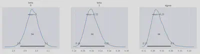
all of the sampled posterior distributions now comfortably enclose their true values within their HPDs.

Closing Remarks

We’ve used the some of the Expectation-Maximisation theory derived in part 1¹ to compute, accurately, the regression coefficients of a simple linear regression model in which a significant proportion of the data has been censored.

As a bonus we saw an alternative way to fit a censored regression model using MCMC and pymc.

References