Huber Regression

Introduction

In my last post about quantile regression post ¹ I touched briefly about least absolute derivation (LAD) regression in order to motivate the pinball loss functioin, but LAD regression is interesting in it’s own right. In this post I’ll discuss the differences between ordinary least squares (OLS) and LAD regression and then move on to an interesting compromise between the two - Huber regression ².

I’m going to use an example dataset I found in the pymc3 documentation ³ to demonstrated the idea.

import pandas as pd
from sklearn.preprocessing import scale
import matplotlib.pyplot as plt

df = pd.DataFrame(
    np.array(
        [
            [1, 201, 592, 61, 9, -0.84],
            [2, 244, 401, 25, 4, 0.31],
            [3, 47, 583, 38, 11, 0.64],
            [4, 287, 402, 15, 7, -0.27],
            [5, 203, 495, 21, 5, -0.33],
            [6, 58, 173, 15, 9, 0.67],
            [7, 210, 479, 27, 4, -0.02],
            [8, 202, 504, 14, 4, -0.05],
            [9, 198, 510, 30, 11, -0.84],
            [10, 158, 416, 16, 7, -0.69],
            [11, 165, 393, 14, 5, 0.30],
            [12, 201, 442, 25, 5, -0.46],
            [13, 157, 317, 52, 5, -0.03],
            [14, 131, 311, 16, 6, 0.50],
            [15, 166, 400, 34, 6, 0.73],
            [16, 160, 337, 31, 5, -0.52],
            [17, 186, 423, 42, 9, 0.90],
            [18, 125, 334, 26, 8, 0.40],
            [19, 218, 533, 16, 6, -0.78],
            [20, 146, 344, 22, 5, -0.56],
        ]
    ),
    columns=["id", "x", "y", "sigma_y", "sigma_x", "rho_xy"],
)
df.drop("id", inplace=True, axis=1)
df.drop("rho_xy", inplace=True, axis=1)
df.head()

x_std, y_std = df.x.std(), df.y.std()
df.x = scale(df.x)
df.y = scale(df.y)

df.sigma_x = df.sigma_x / (2 * x_std)
df.sigma_y = df.sigma_y / (2 * y_std)

_, ax = plt.subplots(figsize=(12, 8))
ax.errorbar(df.x, df.y, df.sigma_y, df.sigma_x, fmt='o')
ax.set(xlim=(-3, 3), ylim=(-3, 3), xlabel='x', ylabel='y');

The data looks like it could, for the most part, have been been generated by some linear process, with the exception of three clear outlying points. We can use statsmodels ⁴ to compute OLS:

import statsmodels.api as sm
ols_fit = sm.OLS(df.y, df.x).fit()

and LAD fits:

lad_fit = sm.QuantReg(df.y, df.x).fit()

and then look at how these behave:

import matplotlib.pyplot as plt

fig, ax = plt.subplots(figsize=(12, 8))

xx = np.linspace(-3, 3, 1000)
ax.errorbar(df.x, df.y, df.sigma_y, df.sigma_x, fmt='o', label='Data')
ax.set(xlim=(-3, 3), ylim=(-3, 3), xlabel=r'$x$', ylabel=r'$y$')
ax.plot(xx, ols_fit.params.values * xx, label='OLS')
ax.plot(xx, lad_fit.params.values * xx, label='LAD')
ax.legend();

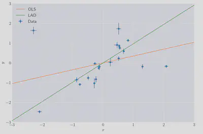
The LAD fit seems quite reasonable. The OLS fit, not so much…

OLS and LAD regression

The OLS regression assumes that each response variable, $y_i$ for $i\in{0, N}$, is a linear functions of the features, $x_i\in\mathbb{R}$. That is,

$$ y_i = \beta_0 + \beta_1 x_i + \epsilon_i. $$

Furthermore it assumes the the noise terms, $\epsilon_i$, are independent of $x_i$ (and one another) and are normally distributed, $\mathcal{N}(0, \sigma^2)$. If we write down the likelihood function, $L$, for this model we have:

\begin{align*} L &= f(x_1, y_1, \ldots, x_N, y_N; \beta, \sigma), \newline L &= \prod_i^N f(x_i, y_i; \beta, \sigma), \newline L &= \prod_i^N \frac{1}{\sqrt{2\pi\sigma^2}} \exp\left(-\frac{(y_i - \beta x_i)^2}{2\sigma^2}\right), \newline \end{align*}

and taking the logarithm to get the log-likelihood, $\mathcal{L}$, we have

\begin{align*} \mathcal{L} &= \sum_i^N\left[-\frac{1}{2}\ln{2\pi\sigma^2} - \frac{(y_i - \beta x_i)^2}{2\sigma^2}\right], \newline \mathcal{L} &= -\frac{1}{2}\sum_i^N\ln{2\pi\sigma^2} - \frac{1}{2\sigma^2}\sum_i^N (y_i - \beta x_i)^2. \end{align*}

where we’ve use the assumed independence of the observations to write the likelihood as a product.

The first term here is a constant with respect to our regression parameter, $\beta$, and so we maximise the log-likelihood by maximising the second term. Clealy this can be achieved with the following:

$$ \hat{\beta} = \operatorname * {argmin} _ {\beta}\sum_i(y_i - \beta x_i)^2. $$

which has a well known analytical solution.

This model is, however, not robust to outlying data i.e. data which violates our assumption about normally distributed residuals. If a dataset we’re trying to fit a regression was generated by a process with a heavy tailed error distribution then we will probably not end up with a good fit to the data.

We can follow a similar argument for LAD regression except using a Laplace distribution for the residuals:

\begin{align*} L = \prod_i^N \frac{1}{2b} \exp\left(-\frac{|y_i - \beta x_i|}{b}\right) \newline \Rightarrow\mathcal{L} = N\ln{2b} - \frac{1}{b}\sum_i^N|y_i - \beta x_i| \end{align*}

The maximimum is then achieved with

$$ \hat{\beta} = \operatorname * {argmin} _ {\beta}\sum_i|y_i - \beta x_i| $$

This time each residual contributes linearly to the loss, rather than quadratically and so outliers have less impact on the fit parameters.

The Huber loss function

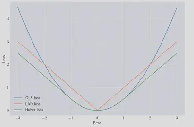
The Huber loss function, $\mathcal{H}$, is a combination of the quadratic OLS loss, and the linear LAD loss. For some $\gamma\in\mathcal{R}$

$$ \mathcal{H}(r_i) = \frac{r_i^2}{2}\text{ if } |r_i| > \gamma\text{ else }\gamma|r_i|-\frac{\gamma^2}{2} $$

where $r_i=y-\hat{y}_ i$ is the residual. I.e. In the Huber loss function the residual contributes linearly if it greater than $\gamma$, and quadratically if is it smaller. We can obviously recover a $|x|$ loss, or a quadratic loss, by taking the limit of small or large gamma (resp.). Motivated by the link between the assumed distributions of the residuals and the resulting loss functions we can think of Huber regression as having a mixture of the two distributions as it’s likelihood, with residuals drawn from a Laplace distribution for large values, and a Gaussian for smaller values.

The shape of this function for $\gamma=1$ is shown below:

We would like to be able to express $\mathcal{H}$ in a more convient form, and luckily it can be expressed as a single expression, in a form which we recognise as a quadratic programme.

$$ \mathcal{H}(r_i) = \min_{z_i\in\mathcal{R}}\frac{z_i^2}{2} + \gamma|r_i - z_i| \equiv \min_{z_i\in\mathcal{R}}\theta(r_i, z_i). $$

To prove these formalutions are equivalent we look to find the minimum of this analytically. Computing the sub-gradients:

\begin{align*} \frac{\partial\theta(r_i, z_i)}{\partial z_i} &= z_i - \gamma = 0 \text{ when } z_i < r_i, \\ \frac{\partial\theta(r_i, z_i)}{\partial z_i} &= z_i + \gamma = 0 \text{ when } z_i > r_i, \\ \frac{\partial\theta(r_i, z_i)}{\partial z_i} &= z_i + \lambda\gamma = 0 \text{ when } z_i = r_i \text{ for } \lambda\in[-1, 1]. \end{align*}

and solving for $z_i$ in each and substituting back in to $\theta(r_i, z_i)$

\begin{align*} \theta (r_i, z_i^{*}) &= \frac{\gamma^2}{2} + \gamma |r_i - \gamma| = \frac{\gamma^2}{2} + \gamma(r_i - \gamma) = -\frac{\gamma^2}{2} + \gamma r_i \text{ when } z_i < r_i, \\ \theta (r_i, z_i^{*}) &= \frac{\gamma^2}{2} + \gamma |r_i + \gamma| = \frac{\gamma^2}{2} - \gamma(r_i + \gamma) = -\frac{\gamma^2}{2} - \gamma r_i \text{ when } z_i > r_i, \\ \theta (r_i, z_i^{*}) &= \frac{r_i^2}{2} \text{ when } z_i = r_i \text{ for } r_i \in [-\gamma, \gamma]. \end{align*}

which matches the original definition of $\mathcal{H}$.

Implementation as a quadratic programme

The L1 norm term in $\mathcal{H}(r_i)$ looks awkward but we can introduce additional variables, $t_i$, and bound them as follows

$$ -t_i \leq r_i - z_i \leq t_i. $$

which is known as the ‘bounding’ trick. There are several other ways to deal with L1 terms in linear programming, all of which are detailed in Erwin Kalvelagen’s blog post on the subject⁵.

We can implement this in gurobi ⁶ as follows

import gurobipy as lp

def huber_regression(
    x: np.array,
    y: np.array,
    gamma: float,
    display: bool=False,
) -> None:

    N = x.shape[0]
    m = lp.Model('Huber Regression')
    m.ModelSense = lp.GRB.MINIMIZE
    beta = m.addVar(name='beta')
    z = m.addVars(N, name='z', lb=-lp.GRB.INFINITY)
    t = m.addVars(N, name='t')
    m.addConstrs((beta * x[i] - y[i] - z[i] <= t[i]) for i in range(N))
    m.addConstrs((beta * x[i] - y[i] - z[i] >= -t[i]) for i in range(N))
    m.setObjective(
        lp.quicksum([0.5 * z[i] * z[i] for i in range(N)]) + gamma * lp.quicksum([t_i for t_i in t.values()])
    )
    m.optimize()
    assert m.status == 2, "Model didn't converge with status {}".format(m.status)
    return m.getVarByName('beta').X

The results of this, compared to the statsmodels OLS and LAD prediction for a few choices for $\gamma$.

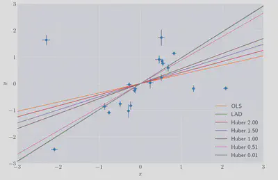
As expected we can see that as $\gamma$ approaches zero the prediction tends towards the LAD prediction and for larger values towards the OLS solution.

Unlike either OLS or LAD regression Huber regression has a hyperparameter we need to choose. Were we working with a larger dataset we could use some ideas like cross-validation to select the value for $\gamma$ which led to the model which generalised the best.

References