Network Discovery with Mixed Integer Programming

Introduction

Mixed integer linear programmes (MIP) are applicable to an amazingly wide range of problems but I’d never considered that you could use them to discover how, given some sort of flow data going into, and out of a set of nodes, MIP could be used to desribe how a series of nodes are interconnected. I came across the idea of network discovery during a Gurobi seminar I attended last year ¹, it was a nice talk so I recommend giving it a watch.

In this post I’ll follow the ideas described in the seminar and develop a MIP model to map out a network topology. In the simplest case I will work with ‘clean’ flow data and then I’ll to extend the model to more tricky situations where we have noisy and/or incomplete datasets. In the later case we’ll need to employ ‘soft’ constraints which are an useful trick to be familiar with.

Linear Programmes and Mixed Integer Programmes

A full description of the theory around linear programmes (LPs) and mixed integer programmes (MIPs) is far beyond the scope of this post but I’ll give a brief overview of what shape these problems take. For a really detailed intoduction to LPs and the more general field of convex optimisation I recommend the Boyd and Vandenberghe book ².

Linear programmes are optimisation problems where the objective function and all constraints are simple linear functions:

\begin{align*} &\min \vec{c}\cdot\vec{x}\newline\text{subject to:}\quad &A\vec{x}=\vec{b},\ \vec{x}\leq\vec{u}. \end{align*}

$\vec x\in\mathbb{R}^n$ are the decision variables, $A\in\mathbb{R}^{n\times m}$ and $b\in\mathbb{R}^m$ are constants which describe the constraints which any proposed solution must satisfy. $c\in\mathbb{R}^n$ is a fixed vector of “costs” which encodes how much each of our decision variables will contribute to the objective. Lastly, $u\in\mathbb{R}^n$ constrains the decision variables themselves.

The $A\vec{x}=\vec{b}$ constraint might seem so restrictive as to limit the amount of interesting problems we can describe, but it turns out that we can model problems which callk for inequalities on $\vec x$ too, we simply need to add in some extra variables (known as “slack” variables) and the problem can once more be writen with an exact quality constraint.

MIPs are an extension of LPs where we further constrain some subset of $x$ to take on integer values. While this might seem like a small extension it makes finding the optimal solutions significantly harder than in the continuous LP case. But in exchange we gain the ability to model much more complex problems, examples of which we’ll see in a moment.

There are many excellent packages for solving LPs and MIPs such as GLPK and CPLEX. Even the python scipy package has built in solvers for LPs. Here I have chosen to use Gurobi ³, mostly because it has a nice python API for building up models and it’s extremely fast at solving these problems.

Network flow as MIP

We will begin by generating some random input and output flow rates, and a random allocation of connections. We will have data telling us the float rates going in at the $n_{\text{input}}$ input nodes, and also how much flow is leaving at each of the $n_{\text{output}}$ nodes.

The true network map is $X\in[0, 1]^{n_{\text{input}}\times n_{\text{output}}}$. $X_{ij} = 1$ means that input node $i$ is connected to output node $j$, $X_{ij} = 0$ means they are not connected. $X$ will not be shown to the MIP optimisation, and our task is to recreate $X$ using only the flow data.

from typing import Tuple
import numpy as np

def generate_flow_allocation_problem(
    n_input: int,
    n_output: int,
    min_flow: float=1,
    max_flow: float=100,
) -> Tuple[np.array, np.array, np.array]:

    X = np.zeros((n_input, n_output))

    # Allocate input nodes randomly to a single output node
    idxs = np.random.randint(n_output, size=n_input)
    for row, idx in enumerate(idxs):
        X[row, idx] = 1

    # Generate some random input rates and use them to compute the true output rates
    rates_in = np.random.randint(min_flow, max_flow, size=n_input).astype(float)
    rates_out = X.T.dot(rates_in).astype(float)

    return X, rates_in, rates_out

X_true, rates_in, rates_out = generate_flow_allocation_problem(10, 10)
print('rates_in', rates_in)
print('rates_out', rates_out)

>>> ('rates_in', array([77., 16., 81., 38., 61., 95., 80., 40., 76., 84.]))
>>> ('rates_out', array([115.,  81., 100.,   0.,  61.,  95.,  40.,  80.,   0.,  76.]))

The decision variables in our MIP are the binary entries of the $X$ matrix and the contraints are that the flow measured at an output node must be equal to the sum of the measured flows at all the input nodes which connect to it. For now our objective function is a constant, since we’re not trying to minimise or maximise anything - our problem only has constraints in it as we’re just trying to find a solution, $X$, which can satisfy the flow constraints:

import gurobipy as lp

def exact_allocation_problem(
    rates_in: np.array,
    rates_out: np.array,
) -> np.array:
    # Make a Gurobi model and turn off all the logging output
    m = lp.Model("exact_allocation")
    m.setParam('OutputFlag', 0)
    n_input, n_output = rates_in.shape[0], rates_out.shape[0]

    # Add the X matrix of variables to the model
    X_vars = m.addVars(n_input, n_output, vtype=lp.GRB.BINARY, name="x")

    # Constrain the flow at the output nodes to equal the sum of connected input nodes
    m.addConstrs(
        lp.quicksum([X_vars[(i, j)] * rates_in[i] for i in range(n_input)]) == rates_out[j]
        for j in range(n_output)
    )

    # Ensure that every input node connects to a single output node
    m.addConstrs(
        lp.quicksum([X_vars[(i, j)] for j in range(n_output)]) == 1
        for i in range(n_input)
    )

    m.setObjective(1)
    m.optimize()

    if m.status == lp.GRB.Status.INF_OR_UNBD:
        raise RuntimeError('Model is infeasible or unbounded')
    elif m.status == lp.GRB.Status.INFEASIBLE:
        raise RuntimeError('Model is infeasible')
    elif m.status == lp.GRB.Status.UNBOUNDED:
        raise RuntimeError('Model is unbounded')

    return np.array(
        [v.x for v in m.getVars() if v.varName.startswith('x[')]
    ).reshape(n_input, n_output)

Gurobi can show us what the model looks like for a small problem:

X_true, rates_in, rates_out = generate_flow_allocation_problem(3, 3)
model, X_pred = exact_allocation_problem(rates_in, rates_out)
model.display()

>>> Minimize
>>>    <gurobi.LinExpr: 1.0>
>>> Subject To
>>>    R0 : <gurobi.LinExpr: 36.0 x[0,0] + 28.0 x[1,0] + 29.0 x[2,0]> = 28.0
>>>    R1 : <gurobi.LinExpr: 36.0 x[0,1] + 28.0 x[1,1] + 29.0 x[2,1]> = 36.0
>>>    R2 : <gurobi.LinExpr: 36.0 x[0,2] + 28.0 x[1,2] + 29.0 x[2,2]> = 29.0
>>>    R3 : <gurobi.LinExpr: x[0,0] + x[0,1] + x[0,2]> = 1.0
>>>    R4 : <gurobi.LinExpr: x[1,0] + x[1,1] + x[1,2]> = 1.0
>>>    R5 : <gurobi.LinExpr: x[2,0] + x[2,1] + x[2,2]> = 1.0
>>> Binaries
>>>    ['x[0,0]', 'x[0,1]', 'x[0,2]', 'x[1,0]', 'x[1,1]', 'x[1,2]', 'x[2,0]', 'x[2,1]', 'x[2,2]']

and given the example data from above

X_pred = exact_allocation_problem(rates_in, rates_out)
print(np.allclose(X_true, X_pred))
>>> True

Neat, we’ve been able to correctly recreate the network map! What about a bigger problem?

X_true, rates_in, rates_out = generate_flow_allocation_problem(20, 20)
X_pred = exact_allocation_problem(rates_in, rates_out)
np.allclose(X_true, X_pred)
>>> False

Ah, something has gone wrong with this one…

np.allclose(X_pred.T.dot(rates_in), rates_out)
>>> True

So the model has managed to find an alternative way of allocating input nodes to output nodes, such that the rates still work out correctly. We need some way to help it to the desired optimal. A few ways to do this:

• Generate more realistic data. Integers between 1 and 100 make it easy to find alternative solutions when the dimension of input and output nodes grows (boring solution - It’d basically sidestepping the issue),
• Tell the model it’s solution isnt correct. If we had some side information about the allocations we could add in extra constraints along the lines of “this input definitely isn’t connected to this output”. But this, too, is cheating! Of course, if we actually had such extra information we could always add it but putting it in afterwards isn’t realistic and still doesn’t mean we’ll get back the true allocations,
• Add more data: If we had a series of input and output flows in some time periods (e.g. the measured daily input/output flows for a week) it will be far less likely there will be alternative optimsal solutions.

The last option is the most interesting so I’ll pursue that idea.

This time generate flow data for $T$ timesteps. I’ll assume that allocations are constant over time, though it would be a fun extension to have time varying networks.

def generate_multiple_time_flow_allocation_problem(
    n_input: int,
    n_output: int,
    n_timesteps: int,
    min_flow: float=1,
    max_flow: float=100,
) -> Tuple[np.array, np.array, np.array]:
    X = np.zeros((n_input, n_output))
    idxs = np.random.randint(n_output, size=n_input)

    for row, idx in enumerate(idxs):
        X[row, idx] = 1

    rates_in = np.random.randint(min_flow, max_flow, size=(n_input, n_timesteps))
    rates_out = X.T.dot(rates_in)

    return X, rates_in.astype(float), rates_out.astype(float)


def exact_allocation_problem_multiple_times(
    rates_in: np.array,
    rates_out: np.array,
) -> np.array:

    m = lp.Model("exact_allocation_multiple_times")
    m.setParam('OutputFlag', 0)
    n_input, n_times = rates_in.shape
    n_output, n_times_ = rates_out.shape
    assert n_times == n_times_

    X_vars = m.addVars(n_input, n_output, vtype=lp.GRB.BINARY, name="x")

    m.addConstrs(
        lp.quicksum([X_vars[(i, j)] * rates_in[i, t] for i in range(n_input)]) == rates_out[j, t]
        for t in range(n_times)
        for j in range(n_output)
    )

    m.addConstrs(
        lp.quicksum([X_vars[(i, j)] for j in range(n_output)]) == 1
        for i in range(n_input)
    )

    m.setObjective(1)
    m.optimize()

    if m.status == lp.GRB.Status.OPTIMAL:
        print('Optimal objective: %g' % model.objVal)
    elif m.status == lp.GRB.Status.INF_OR_UNBD:
        print('Model is infeasible or unbounded')
    elif m.status == lp.GRB.Status.INFEASIBLE:
        print('Model is infeasible')
    elif m.status == lp.GRB.Status.UNBOUNDED:
        print('Model is unbounded')

    return np.array(
        [v.x for v in m.getVars() if v.varName.startswith('x[')]
    ).reshape(n_input, n_output)

Now we can generate a problem with lots of flows, and see how many timesteps worth of data the model needs until it finds the right map:

X_true, rates_in, rates_out = generate_multiple_time_flow_allocation_problem(50, 50, 6)
for time_steps in range(6):
    limited_rates_in, limited_rates_out = rates_in[:,:time_steps], rates_out[:,:time_steps]
    X_pred = exact_allocation_problem_multiple_times(limited_rates_in, limited_rates_out)
    print(np.allclose(X_pred, X_true))

>>> False
>>> False
>>> True
>>> True
>>> True
>>> True

Cool, even for large systems we can reproduce the correct network if we have enough measurements.

Adding some noise

What would happen if we jittered the flow data a little, to make it look a bit more realistic

X_true, rates_in, rates_out = generate_flow_allocation_problem(20, 20)
rates_in += np.random.normal(0, 5, rates_in.shape)
X_pred = exact_allocation_problem(rates_in, rates_out)
...
RuntimeError: Model is infeasible

Actually this is completely expected. Our model is using equality constraints which are extremely unlikely to be simultaneously satisfied once we applied some noise to the data. We have to relax these constraints into “soft constraints” - constraints which are allowed to be violated, but to do so we must pay a penalty.

Let’s rewrite each “conservation of flow” constraint by splitting it into two inequalities:

\begin{align*} &\sum_i X_{ij}I_i - f_{jt} \leq O_{jt}, \quad f_{jt} \geq 0 \ \ \forall j, t \quad (1) \newline &\sum_i X_{ij}I_i + f_{jt} \geq O_{jt}, \quad f_{jt} \geq 0 \ \ \forall j, t \quad (2) \newline \end{align*}

where $I_i$ and $O_i$ are the input and output flows respectively. Note that if rather than $f_{jt} \geq 0$ we had an equality constraint $f_{jt} = 0$ we would recover the “exact” model from above.

How do these constraints work in practise? If we’ve lost some of the input we will have $\sum_i X_{ij}I_i \leq O_{jt}$ for some $j$ and $t$. Constraint (1) is therefore satisfied for all values of $f_{jt}$ but constraint (2) will require $f_{jt}$ to be at least the value of the discrepancy between the sum of inputs for a given allocation and the output. Conversely, if the measurement of output is higher than the true value constraint (2) is trivially satisfied and constraint (2) is the active one, again resulting in the value of $f_{jt}$ being at least the value of the size of the error. I.e. these constraints make $f_{jt}$ a lower bound on the absolute value of the input-output mismatch for connection $j$ at time $t$.

With these new constraints we now change the objective we can now encourage the model to minimise these violating terms $f_{jt}$ by changing the model to minimise $\sum_{jt} f_{jt}$.

This approach treats all of the constraints uniformly (i.e. the sum over $f$’s has no weighting), but if some connections were more important than others we could introduce a constant weighting, $w_j$, and instead minimise $\sum_{jt} w_jf_{jt}$.

Let’s build this model and check that is works as we expect:

def fuzzy_allocation_problem_multiple_times(
    rates_in: np.array,
    rates_out: np.array,
) -> Tuple[np.array, np.array]:
    m = lp.Model('fuzzy_allocation_multiple_times')
    m.setParam('OutputFlag', 0)
    n_input, n_times = rates_in.shape
    n_output, n_times2 = rates_out.shape
    assert n_times == n_times2

    X_vars = m.addVars(n_input, n_output, vtype=lp.GRB.BINARY, name="x")

    f_terms = m.addVars(n_output, n_times, lb=0.0, vtype=lp.GRB.CONTINUOUS, name="f")

    for t in range(n_times):
        for j in range(n_output):
            combined_flow_in = lp.quicksum([X_vars[(i, j)] * rates_in[i, t] for i in range(n_input)])
            m.addConstr(combined_flow_in - f_terms[(j, t)] <= rates_out[j, t])
            m.addConstr(combined_flow_in + f_terms[(j, t)] >= rates_out[j, t])

    for i in range(n_input):
        m.addConstr(lp.quicksum([X_vars[(i, j)] for j in range(n_output)]) == 1)

    m.setObjective(lp.quicksum(f_terms))
    m.optimize()

    if m.status == lp.GRB.Status.INF_OR_UNBD:
        raise RuntimeError('Model is infeasible or unbounded')
    elif m.status == lp.GRB.Status.INFEASIBLE:
        raise RuntimeError('Model is infeasible')
    elif m.status == lp.GRB.Status.UNBOUNDED:
        raise RuntimeError('Model is unbounded')

    X_pred = np.array(
        [v.x for v in m.getVars() if v.varName.startswith('x[')]
    ).reshape(n_input, n_output)

    f_terms = np.array([
        m.getVarByName('f[{},{}]'.format(j, t)).x
        for j in range(n_output)
        for t in range(n_times)
    ]).reshape(n_output, n_times)

    return X_pred, f_terms

X_true, rates_in, rates_out = generate_multiple_time_flow_allocation_problem(50, 50, 5)
rates_in += np.random.normal(0, 2, rates_in.shape)
rates_out += np.random.normal(0, 2, rates_out.shape)
X_pred, f_terms = fuzzy_allocation_problem_multiple_times(rates_in, rates_out)
print(np.allclose(X_pred, X_true))
>>> True

We can check the distribution of the error terms to check that they are mostly quite small:

from scipy import stats

_, ax = plt.subplots(figsize=(15, 10))

xx = np.linspace(0, 12, 100)
ax.hist(f_terms, density=True, label=r'$f_{jt}$')
ax.plot(xx, stats.norm(0, 2).pdf(xx), label='Noise term')
ax.set(xlim=(0, 10), xlabel=r'$f_{jt}$', ylabel='Density')
ax.legend();

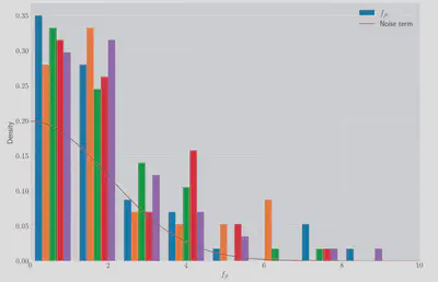
Where the ‘Noise term’ is a Gaussian PDF with the variance the same as I added to the true flow rates and is shown for scale.

Closing Remarks

We’ve used Gurubi to implement and solve a MIP which allows us to correctly identify an unknown set of connections in a simple network. We then extended this to more realistic situations with a noisy data set, using soft constraints rather than exact constraints to keep the model feasible.

References