Quantile Regression

Introduction

Given some covariates, $X$, and a dependent variable, $y$, ordinary least squares regression (OLS) provides a value for the expectated value $\mathbb{E}[Y|X]$ but this is not always sufficient. Often we want to know more about the full conditional distribution, $y|x$. There are a number of ways we can go about doing this but here I will focus on extracting more information about the distribution by estimating its $\tau$-th quantile, $Q_{\tau }(Y|X)$, where $0\le \tau \le 1$.

To demonstrate this I’ll use the LIDAR dataset from the book ‘All of Nonparametric Statistics’ ¹ shown here

import matplotlib.pyplot as plt
import pandas as pd
from sklearn import preprocessing

df = pd.read_csv(
    'http://www.stat.cmu.edu/~larry/all-of-nonpar/=data/lidar.dat',
    sep='\s+',
    skiprows=1,
    names=['range', 'logratio'],
)
df[['range', 'logratio']] = preprocessing.scale(df)

_, ax = plt.subplots(figsize=(12, 8))
ax.scatter(df.range, df.logratio)
ax.set(xlabel='range', ylabel='logratio');

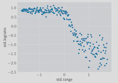
The actual meaning of the data won’t matter so much for what follows, all we need to know is that we need to predict the logratio using only the range feature. If you’re interested there is some explanatory documentation here ¹.

It’s an interesting dataset displaying non-linearity as well as heteroskedasticity. We can deal with the non-linearity easily enough and just focus on predicting the central value, but what if we’re interested in producing prediction intervals for any given range value?

LAD regression

We’ll approach the problem of computing a general quantile by focusing on one, the median. Least absolute deviations (LAD) regression minimises the mean of the absolute values of the residuals:

$${\mathcal{L}}_1=\frac{1}{N}\sum _{i=0}^N|y_i-{\hat{y}}_i|.$$

where ${\hat{y}}_i$ is the $i$-th predicted $y$ value.

While the OLS regression gives us the mean of the conditional distribution $Y|X$, LAD regression will give us it’s median, or the $\tau =0.5$ quantile. This is quite easy to motivated if we zoom in on a thin slice of the $x$ value, range, in the above data, effectively compressing the regression problem down to one of choosing a single correct logratio value, with no gradient.

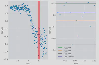
For this small region we can treat the $x_i$ to be a constant, and our prediction is now just a single value, $\beta$. We can then differentiate the objective, ${\mathcal{L}}_1$, explicitly:

$$\frac{d{\mathcal{L}}_1}{d\beta }=\frac{1}{N}\sum _{i=0}^N\frac{y_i-\beta }{|y_i-\beta |}=-\frac{1}{N}\sum _{i=0}^N\text{sign}(y_i-\beta )=0.$$

where the $\text{sign}$ function is +1 if the argument is positive and -1 if it’s negative. The optimial solution is clearly when half of the residuals, $y_i-\beta$, are positive and half are negative, i.e. when $\beta$ is the median.

LAD regression has a lot of interesting properties in it’s own right (as well as some cool solutions using mixed integer programming) but that is for another time. For now we’ve seen enough of an introduction to motivate the more general form.

The Pinball Loss

The ‘pinball’ loss, also known as the ‘check’ function, is defined as follows

$${\rho }_{\tau }(r_i)=r_i(\tau -\text{I}(r_i<0)).$$

where $r_i$ is our $i^{\text{th}}$ residual and $\text{I}$ is the indicator function. If we pick $\tau =0.5$ we can express this as

$${\rho }_{\tau }(r_i)=\frac{r_i}{2}\text{ if }{r}_i>0\text{ else }-\frac{r_i}{2}=\frac{|r_i|}{2}\sim |r_i|$$

so pinball is a special case of the L1 loss. It turns out other values of $\tau$ pick out other quantile values, e.g. $\tau =0.1$ is the 10th percentile, $\tau =0.25$ is the 1st quartile etc. This is quite straightforward to prove.

For fixed $x$ (our range values) we want to minimise our expected loss over all the possible values of the random variable $Y$ (logratio). Let $F_Y(y)=\mathbb{P}(Y<y)$ be the CDF of the dependent variable. Our goal then is to minimise the expected loss over $\hat{y}$:

$$\begin{array}{rl}\mathbb{E}[{\rho }_{\tau }(Y-\hat{y})]& ={\int }_{-\mathrm{\infty }}^{\mathrm{\infty }}{\rho }_{\tau }(y-\hat{y})d{F}_Y(y)\\ & =(\tau -1){\int }_{-\mathrm{\infty }}^{\hat{y}}(y-\hat{y})d{F}_Y(y)+\tau {\int }_{\hat{y}}^{\mathrm{\infty }}(y-\hat{y})d{F}_Y(y)\end{array}$$

where we’ve split the integral into two ranges, one for each case in the loss function. We differentiate this using Richard Feynman’s favourite trick ² (the Leibniz integral rule):

$$\begin{array}{rl}\frac{d}{dx}{\int }_{a(x)}^{b(x)}f(x,t)dt=& f(x,b(x))\frac{d}{dx}b(x)-f(x,a(x))\frac{d}{dx}a(x)+\\ & {\int }_{a(x)}^{b(x)}\frac{\partial }{\partial x}f(x,t)dt.\end{array}$$

Using this we get

$$\begin{array}{rl}\frac{d\mathbb{E}[{\rho }_{\tau }(Y-\hat{y})]}{d\hat{y}}=(\tau -1)& [(y-\hat{y}){|}_{y=\hat{y}}-{\int }_{-\mathrm{\infty }}^{\hat{y}}d{F}_Y(y)]+\\ \tau & [-(y-\hat{y}){|}_{y=\hat{y}}-{\int }_{\hat{y}}^{\mathrm{\infty }}d{F}_Y(y)]=0\end{array}$$

$$\begin{array}{r}\Rightarrow -\tau ({\int }_{-\mathrm{\infty }}^{y_{\tau }}d{F}_Y(y)+{\int }_{y_{\tau }}^{\mathrm{\infty }}d{F}_Y(y))+{\int }_{-\mathrm{\infty }}^{y_{\tau }}d{F}_Y(y)=0,\end{array}$$

$$\begin{array}{r}\Rightarrow \tau =F_Y(y_{\tau })\end{array}$$

where we’ve used the fact that the integral of any CDF over all values is just one and defined $y_{\tau }$ to be the $y$ value at which the derivative of the expectation is zero. By it’s definition $F_Y(y_{\tau })$ is the ${\tau }^{\text{th}}$ quantile of $Y$ and so we have shown that the pinball loss is the correct choice to pick out the quantiles we are interested in when performing regressions.

Quantile Regression with Pytorch

We’ve got enough theory to get back to the example dataset. I’m going to use a simple multi-layer perceptron (MLP) neural network to perform the regression. One possible way to build this model would be to have a network output predict a quantile, and then train a model for each quantile we want. Instead, I’m going to have the last layer of the network output multiple values value, one for each quantile, and train them all in parallel. The only disadvantage of this approach is that were we to change our minds about which quantiles we’re interested in we’d have to train the whole model again.

Starting by defining the loss and the MLP using pytorch:

import torch
import torch.nn as nn
from torch.optim import Adam

def pinball_loss(quantile_predictions, target, quantiles):
    pinball = lambda tau, residual: torch.max((tau - 1) * residual, tau * residual).unsqueeze(1)
    losses = [
        pinball(tau, target - quantile_predictions[:, i])
        for i, tau in enumerate(quantiles)
    ]
    return torch.mean(torch.sum(torch.cat(losses, dim=1), dim=1))

class QuantileModel(nn.Module):
    def __init__(self, quantiles, n_hidden=32):
        super().__init__()
        self.model = nn.Sequential([
            nn.Linear(1, n_hidden),
            nn.Sigmoid(),
            nn.Linear(n_hidden, n_hidden),
            nn.Sigmoid(),
            nn.Linear(n_hidden, quantiles.shape[0]),
        ])

    def forward(self, x):
        return self.model(x)

and then training the model using a souped-up version of stochastic gradient descent, ADAM:

import numpy as np

x = df.range.values.reshape(221, 1)
y = df.logratio.values

quantiles = np.linspace(0.05, 0.95, 10)
net = QuantileModel(quantiles, 32)

optimizer = Adam(net.parameters(), lr=0.1)

epochs = 200
losses = []

for e in range(epochs):
    optimizer.zero_grad()
    preds = net(torch.from_numpy(x).float())
    loss = pinball_loss(preds, torch.from_numpy(y).float(), quantiles)
    loss.backward()
    losses.append(loss)
    optimizer.step()

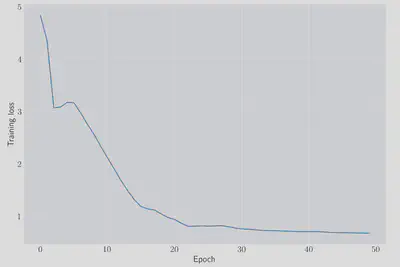
We can check that the network has managed to learn something by looking at the value of the loss function as we train:

fig, ax = plt.subplots(figsize=(12, 8))
ax.plot(losses)
ax.set(xlabel='epoch', ylabel='training loss');

and we can look at the network’s predictions for the quantiles we trained on:

fig, ax = plt.subplots(figsize=(12, 8))

xx = torch.linspace(df.range.min(), df.range.max(), 100).reshape(-1, 1)
yy = net(xx).detach().numpy()

for idx, q in enumerate(quantiles):
    plt.plot(xx, yy[:, idx], 'b-', alpha=0.2)

ax.plot(x, y, 'b.')
ax.plot(xx, yy[:,5], 'r-', label='Median prediction')
fill_quantiles = lambda y0, y1, label, alpha: \
    ax.fill_between(xx.reshape(-1), y0, y1, alpha=alpha, color='blue', label=label)
fill_quantiles(yy[:,2], yy[:,-3], '25%-75% region', 0.3)
fill_quantiles(yy[:,0], yy[:,-1], '5%-95% region', 0.1)
ax.set(xlabel='range', ylabel='logratio')
ax.legend();

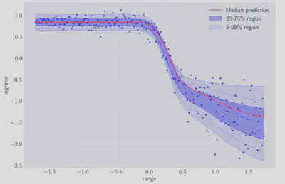
Even without tuning any of the model parameters we can see we are getting a reasonable fit. We can also look in more detail at the distribution of logratio for particular values of range:

fig, ax = plt.subplots(figsize=(12, 8), ncols=3)
min_, max_ = 1e6, -1e6
for a, range_ in zip(ax, np.array([-1.5, 0.45, 1.5])):
    predictions = net(torch.from_numpy(np.array([range_])).reshape(1, -1).float()).detach().numpy().squeeze()
    min_ = min(min_, predictions.min())
    max_ = max(max_, predictions.max())
    a.plot(
        quantiles,
        predictions,
        marker='x',
        label=f'range = {range_}',
    );

ax[0].set(ylabel='logratio')
[a.set(xlabel='quantile') for a in ax]
[a.set(ylim=(min_, max_)) for a in ax]
[a.legend() for a in ax];

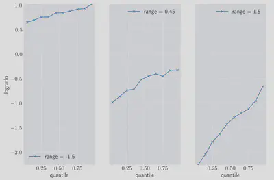
Once again we can see that not only are we capturing the change in the central value of the data, but also it’s heteroskedastic nature since the conditional distribution covers a wider range of logratio values at higher ranges.

Closing Remarks

We motivated the pinball loss by looking briefly at the LAD regression obective function, and then proved that the pinball loss can pick out whatever quantile we are interested in based on the $\tau$ value. We then used this loss function to train a simple neural network to predict some quantiles of the LIDAR dataset.

References