Efficient timeseries joins with pyspark
Introduction
Time series data is very common. The obvious way such data arises is when measurements of a quantity (quantities) are taken repeatedly over time, leading to scalar (vector) timeseries. But another interesting example comes when working with event-driven software architectures. In these systems components communicate to one another using one or more asynchronous ‘streams’ of data (think redis pubsub, kafka etc.). In my experience at Gambit Research these streams can be used to drive some kind of decision making such as an automated trading system, and in that case these streams of information will also be useful to researchers.
In this post I’ll use pyspark to build two toy timeseries and show how the join can be done in two different ways. Both will give the same results, but the performance will scale very differently.There are a lot of similar shaped questions to the one posed above which the optimisation discussed here will apply to. But for the concreteness I’ll pick this one:
Get me every message on stream
This approach is similar to the deltalake optimisation shown in [1]. See also, a nice scala version here [2].
Generating timeseries data
Let’s jump straight into some code - we want a function to generate timestamped entries for our stream, with some associated feature which the message on the stream carried. The features can be discrete or continuous.
import pyspark
from pyspark.sql import functions as F
from pyspark.sql import types as T
from typing import Optional


class FeatureType:
    Discrete = 1
    Continuous = 2


discrete_values = F.array([F.lit(v) for v in ("A", "B", "C")])


def generate_time_series(
    name: str,
    n: int,
    inter_event_ms: float = 10e3,
    now_ms: Optional[float] = None,
    noise: Optional[pyspark.sql.column.Column] = F.lit(0),
    feature_type: FeatureType = None,
) -> pyspark.sql.DataFrame:
    if now_ms is None:
        now_ms = 1000 * F.unix_timestamp(F.current_timestamp())

    spark_df = spark.range(0, n).select(
        F.col("id").alias(f"{name}_id"),
        (now_ms - inter_event_ms * F.col("id") + noise)
        .cast(T.LongType())
        .alias(f"{name}_time_ms"),
    )

    if feature_type is None:
        pass
    elif feature_type == FeatureType.Discrete:
        spark_df = spark_df.withColumn(
            f"{name}_value",
            discrete_values.getItem((3 * F.rand()).cast("int")),
        )
    elif feature_type == FeatureType.Continuous:
        spark_df = spark_df.withColumn(f"{name}_value", 10 * F.randn())
    else:
        raise

    return spark_df
Hopefully it’s fairly self explanatory but in summary:
spark_dfis built by making an index column,id, from 1 ton,- The ’time’ column is generated by hopping backwards in time by a fixed amount with some (optional) user-defined noise term,
- The ‘value’ column is just meant to encode some information carried by the stream of messages.
If you’re not familiar with spark dataframes you can think of them as being broadly similar to pandas dataframes. One difference to pandas which tends to surprise people new to spark is that everything is executed lazily. That is, no actually computation is done until the result is required. So, for example, I can run generate_time_series with a huge value for n and the result will return almost immediately:
n = 1000000000000000
start = time.time()
ts = generate_time_series("ts", n)
end = time.time()
print(end - start)
>>> 0.04685831069946289
The fact that a laptop can run this without grinding to a halt (or the python process getting OOM killed if you’re lucky [3]) should also be a clue that spark hasn’t actually built this dataset.
Similarly to the postgres ’explain’ command We can ask spark to tell us it’s plan to perform the tasks we’re specified, for simple things like creating a new dataframe this won’t be interesting, but later on we will see that, depending on the way we phrase the problem to spark, it will take very different routes to the same result:
ts.explain()
>>> == Physical Plan ==
>>> *(1) Project [id AS ts_1_id, cast(((1.616365207E12 - (cast(id as double) * 10000.0)) + 0.0) as bigint) AS ts_1_time]
>>> +- *(1) Range (0, 1000000000000000, step=1, splits=64)
If you were to do something to spark_df which required actually knowing it’s contents (such as converting it to a pandas dataframe or writing it to disk) spark would go through this plan and create.
To play around with joining two timeseries at different scales we’ll use the function:
def generate_series(n: int):
    now_ms = int(1000 * time.time())
    return (
        generate_time_series(
            "ts_1",
            n,
            now_ms=now_ms,
            noise=2000 * F.randn(),
            feature_type=FeatureType.Discrete,
        ),
        generate_time_series(
            "ts_2",
            n,
            now_ms=now_ms,
            noise=5000 * F.randn(),
            feature_type=FeatureType.Continuous,
        ),
    )
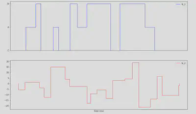
A small sample of these timeseries looks as follows:
Using a regular join
Easy, use the spark dataframe join method, specifying our constraints on the time variables as part of the join:
ts_1, ts_2 = generate_series(N)
window_ms = 10000

conditions = (
   (ts_1.ts_1_time >= ts_2.ts_2_time - window_ms) &
   (ts_1.ts_1_time <= ts_2.ts_2_time + window_ms)
)

joined = ts_1.join(ts_2, conditions)
The output of explain for joined is:
== Physical Plan ==
BroadcastNestedLoopJoin BuildRight, Inner, ((ts_1_time >= (ts_2_time - 10000)) AND (ts_1_time <= (ts_2_time + 10000)))
:  *(1) ...build ts_1
+- BroadcastExchange IdentityBroadcastMode
  +- *(2) ...build ts_2
(I’ve redacted the bits we’ve already seen above which specify how to build ts_(1|2) for readability). The interesting bit here is BroadcastNestedLoopJoin - spark has several strategies for performing joins and this is one them. The ’nested loop’ portion of the name is telling us that something akin to
for row_1 in ts_1:
	for row_2 in ts_2:
		if join_condition(row_1, row_2):
			...
is going to be run. The ‘broadcast’ part requires a little understanding of how spark distributes work which is beyond the scope of this; but roughly speaking it means that spark will try not to copy both datasets to every spark worker, instead it’ll build ts_1 (for example) such that it’s split up across workers, and only copy ts_2 across all the workers.
If we scale the job to make the timeseries larger by increasing N we can see that spark will change its plan - though it’s worth noting that the point at which spark will swap between approaches will depend on how it’s configured and maybe even the size of the cluster it’s being run on so your mileage may vary. For my setup
== Physical Plan ==
CartesianProduct ((ts_1_time >= (ts_2_time - 10000)) AND (ts_1_time <= (ts_2_time + 10000)))
:  *(1) ...build ts_1
   *(2) ...build ts_2
CartesianProduct is the same as BroadcastNestedLoopJoin but spark can’t even save us from copying both datasets across all the workers. This will scale quadratically in the number of rows in our timeseries and will therefore be completely impractical for any real-world datasets.
The ‘bucketed’ approach
A more efficient approach is to divide up the time range over which we are interested into buckets. Each datapoint in the first data frame gets assigned to a single bucket, each datapoint in the second dataframe gets a copy one for every bucket that the ‘join window’ spans or, in code:
def time_series_join(
    x: pyspark.sql.DataFrame,
    y: pyspark.sql.DataFrame,
    t: pyspark.sql.column.Column,
    start: pyspark.sql.column.Column,
    stop: pyspark.sql.column.Column,
    bucket_size: int,
):
    x = x.withColumn("_bucket", (t / bucket_size).cast("bigint"))
    y = y.withColumn(
        "_bucket",
        F.explode(
            F.sequence(
                (start / bucket_size).cast("bigint"),
                (stop / bucket_size).cast("bigint"),
            )
        ),
    )
    return x.join(
        y, [x["_bucket"] == y["_bucket"], t >= start, t <= stop], how="inner"
    ).drop("_bucket")


res = time_series_join(
    events,
    measurements,
    t=F.col("event_time"),
    start=F.col("measurement_time") - window_ms,
    stop=F.col("measurement_time") + window_ms,
    bucket_size=window_ms,
)
The spark join still has our two inequality constraints on the times as before, but we now have an addition equality constraint that the buckets have to match across the dataframes. This will make it easier for spark to optimise the join as we can see from sparks plan:
== Physical Plan ==
SortMergeJoin [_bucket], [_bucket], Inner, ((ts_1_time >= (ts_2_time - 10000)) AND (ts_1_time <= (ts_2_time + 10000)))
:- *(2) Sort [_bucket ASC NULLS FIRST], false, 0
:  +- Exchange hashpartitioning(_bucket, 128), true
:     +- *(1) Project [ts_1_id, ts_1_time, ts_1_value, cast((cast(ts_1_time as double) / 10000.0) as bigint) AS _bucket]
:        +- ...build ts_1
+- *(4) Sort [_bucket ASC NULLS FIRST], false, 0
  +- Exchange hashpartitioning(_bucket, 128), true
     +- Generate explode(sequence(cast((cast((ts_2_time - 10000) as double) / 10000.0) as bigint), cast((cast((ts_2_time + 10000) as double) / 10000.0) as bigint), None, Some(UTC))), [ts_2_id, ts_2_time, ts_2_value], false, [_bucket]
        +- ...build ts_1
SortMergeJoin is a more efficient join strategy than the fearful CartesianProduct from before and so you can expect significantly increased performance.
References
[1] https://docs.databricks.com/delta/join-performance/range-join.html
[2] http://zachmoshe.com/2016/09/26/efficient-range-joins-with-spark.html
Jack Medley
Head of Research, Gambit Research
Interested in programming, data analysis, optimisation and Bayesian statistics